
Overview
For an overview of the Liver toxicity dataset.
Independent PCA analysis
Independent Principal Component Analysis (IPCA) combines the advantages of both PCA and Independent Component Analysis (ICA). It uses ICA as a denoising process of the loading vectors produced by PCA to better highlight the important biological entities and reveal insightful patterns in the data. A sparse version is also proposed (sIPCA).
data(liver.toxicity)
X <- liver.toxicity$gene
dose <- liver.toxicity$treatment[,3]
dose[(dose == 50) | (dose == 150)] <- 'low'
dose[(dose == 1500) | (dose == 2000)] <- 'high'
time <- liver.toxicity$treatment[,4]
dose.time = as.facor(paste(dose, time, sep = '-'))

## IPCA
result <- ipca(X, ncomp = 3, mode="deflation", scale = FALSE)
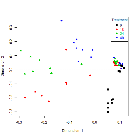
Samples representation
col <- as.numeric(as.factor(time))
plotIndiv(result, ind.names = times, cex = 0.5, col = col)

## Add legend
legend("topright", legend = unique(col), col = unique(col),
       text.col = unique(col), title = "Treatment"))
We have often found that IPCA offers a better visualization of the data than ICA and with a smaller number of components than PCA. IPCA works well if the data have a super-Gaussian distribution.
Understanding Kurtosis
The kurtosis measure is used to order the loading vectors to order the Independent Principal Components. We have shown that the kurtosis value is a good post hoc indicator of the number of components to choose, as a sudden drop in the values corresponds to irrelevant dimensions.
result$kurtosis
[1] 10.6698119   7.2159542   0.5875141